1. Introduction

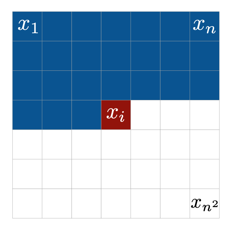
Pixel CNN was proposed in Oord et al. 2016 and is an auto-regressive generative model. It is effectively an auto encoder that honors the auto-regressive property using masked convolutions. The data consists of a set of images, \(\mathcal{D} = \{\pmb{x}^{(t)}\}_{t=1}^T \text{ where } \pmb{x}_i \in \mathbb{R}^{c\times n\times n}\) and T = number of examples, c = channels, and n = height = width of an image. The goal is to learn the joint distribution over all pixels using the chain rule of probability:

The value \(p(x_i|x_1,...,x_{i-1})\) is the likelihood of the ith pixel, \(x_i\), given the previous pixels \(x_1,..., x_{i-1}\). Pixels are conditioned in a row-by-row pixel-by-pixel fashion which is highlighted in Figure 1.

Moving forward, we will step through how to train a Pixel CNN on both black and white images and color images using Pytorch. All code reviewed in this post can be found at this GitHub repo. It should be noted that this blog post was inspired after I completed homework 1 of Berkeley's Deep Unsupervised Learning Course. While my Pixel CNN implementation is not identical to their solution, I do borrow their datasets and some helper methods.

2. Loading MNIST Dataset

In the repo you will find a pickled dictionary data/mnist.pkl. The keys 'train' and 'test' will map you to the train and test numpy array of images, respectively. Each image is of shape (28, 28, 1) and takes on value between [0, 255]. To simplify the problem, we will make the images binary by assigning pixels values > 127.5 value 1 and all other pixels value 0. We then will create a Pytorch Dataset and DataLoader where a given batch will be of shape (128, 1, 28, 28) and contains 'x' and 'y' tensors. The 'x' tensor is a batch of images normalized to 0 mean 1 std and the 'y' tensor is a batch of ground truth binary images.

import torch
from torch.utils.data import Dataset, DataLoader
import numpy as np
import pickle

class Data(Dataset):
    def __init__(self, array, device='cpu', mean=None, std=None):
        self.N, self.H, self.W, self.C  = array.shape
        self.ttl_dims = self.C * self.H * self.W
        self.array = array
        self.device = device
        if mean is None and std is None:
            self.mean = np.mean(self.array, axis=(0,1,2))
            self.std = np.std(self.array, axis=(0,1,2))
        else:
            self.mean = mean
            self.std = std

    def __len__(self):
        return self.N
    
    def __getitem__(self, idx):
        if torch.is_tensor(idx):
            idx = idx.item()
        
        x = self.array[idx].copy().astype(float)
        for i in range(self.C):
            x[:,:,i] = (x[:,:,i] - self.mean[i])/self.std[i]

        return {
            'x': torch.tensor(x, dtype=torch.float).to(self.device).permute(2, 0, 1),
            'y': torch.tensor(self.array[idx], dtype=torch.long).to(self.device).permute(2, 0, 1)}
    
    @staticmethod
    def collate_fn(batch):
        bsize = len(batch)

        return {
            'x': torch.stack([batch[i]['x'] for i in range(bsize)], dim=0).contiguous(),
            'y': torch.stack([batch[i]['y'] for i in range(bsize)], dim=0).contiguous()}
    
    @staticmethod
    def read_pickle(fn, dset):
        assert dset=='train' or dset=='test'
        with open(fn, 'rb') as file:
            data = pickle.load(file)[dset]
            if 'mnist.pkl' in fn:
                data = (data > 127.5).astype('uint8')

            return data

train_arr, test_arr = Data.read_pickle('data/mnist.pkl', 'train'), Data.read_pickle('data/mnist.pkl', 'test')
train = DataLoader(
    Data(train_arr), batch_size=128, shuffle=True, collate_fn=Data.collate_fn)
test = DataLoader(
    Data(test_arr, mean=train.dataset.mean, std=train.dataset.std), 
    batch_size=128, shuffle=True, collate_fn=Data.collate_fn)

for batch in train:
    print(type(batch))
    print(batch['x'].shape)
    print(batch['y'].shape)
    break

Output:

    <class 'dict'>
    torch.Size([128, 1, 28, 28])
    torch.Size([128, 1, 28, 28])
    

3.0 Pixel CNN Binary Images

Now we will begin to open up the Pixel CNN architecture. We will review each component in the architecture which is highlighted in the below figures. Note, the below architecture is almost identical to the one in the original paper. The only differences are we use a Conv 7x7 in the residual block (as opposed to 3x3), and we use 64 convolution filters.

3.1 Masked Convolution

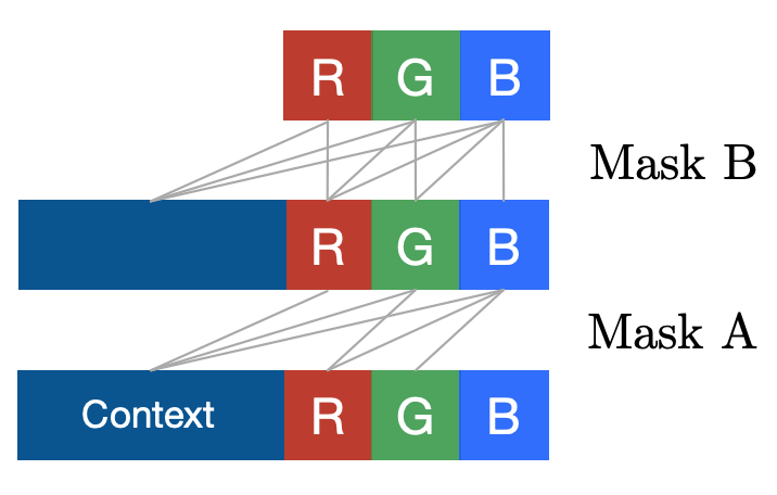
As a convolution kernel traverses through the input image, \(\pmb{x}\), we need to apply a mask to the kernel to ensure pixels to the left and above the current pixel are only used in the convolution operation. This is referred to as the context and is highlighted in Figure 1. Below we will show how to generate the different types of masks, A and B.

3.1.1 Mask Type A Single Channel

One neat thing about this architecture is the width and height of the input image will be maintained across all layers within the network. For simplicity, let's assume an input image of shape 5x5 with one channel and kernel size of 3x3. Next, use the below formula to determine how much we need to pad our input image to maintain the same width/height:

Next, we need to apply a mask to our kernel to honor the auto-regressive property. Figure 4 shows the masked convolution operation for this toy example.

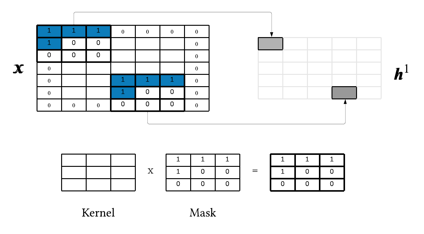
Hopefully it is clear that each stride of the convolution is auto-encoding the current pixel, \(x_i\). We mask our kernel because all pixels to the right and below the current pixel essentially do not exist at inference time. Finally, the reason this is Mask A is because \(h_i^1 = f(\pmb{x}_{< i})\), i.e. a given pixel in the hidden state is a function of the only the context.

3.1.2 Mask B Single Channel

In the case of Mask B, \(h_i^l = f(h_i^{l-1}, \pmb{h}_{< i}^{l-1})\), i.e. a given pixel in the hidden state is a function of both the context and the current pixel being auto-encoded. As a result, below is mask type B for this toy example:

3.1.3 Masked Convolution Pytorch Single Channel

It is actually pretty simple to implement masked convolution into Pytorch, see below:

class MaskedConv2dBinary(Conv2d):
    def __init__(self, m_type, in_channels, out_channels, kernel_size, padding):
        assert m_type=='A' or m_type=='B'
        super().__init__(
            in_channels=in_channels, out_channels=out_channels, kernel_size=kernel_size, stride=1, padding=padding)
        self.register_buffer('mask', torch.zeros_like(self.weight))

        if m_type=='A':
            self.mask[:, :, 0:kernel_size//2, :] = 1
            self.mask[:, :, kernel_size//2, 0:kernel_size//2] = 1
        else:
            self.mask[:, :, 0:kernel_size//2, :] = 1
            self.mask[:, :, kernel_size//2, 0:kernel_size//2 + 1] = 1
    
    def forward(self, x):
        self.weight.data *= self.mask
        
        return super().forward(x)

conv_a = MaskedConv2dBinary('A', 1, 64, 7, 3)
print('Mask A')
print(conv_a.mask[0,:,:,:])

conv_b = MaskedConv2dBinary('B', 64, 64, 7, 3)
print('Mask B')
print(conv_b.mask[0,0,:,:])

Output:

        Mask A
        tensor([[[1., 1., 1., 1., 1., 1., 1.],
                    [1., 1., 1., 1., 1., 1., 1.],
                    [1., 1., 1., 1., 1., 1., 1.],
                    [1., 1., 1., 0., 0., 0., 0.],
                    [0., 0., 0., 0., 0., 0., 0.],
                    [0., 0., 0., 0., 0., 0., 0.],
                    [0., 0., 0., 0., 0., 0., 0.]]])
        Mask B
        tensor([[1., 1., 1., 1., 1., 1., 1.],
                [1., 1., 1., 1., 1., 1., 1.],
                [1., 1., 1., 1., 1., 1., 1.],
                [1., 1., 1., 1., 0., 0., 0.],
                [0., 0., 0., 0., 0., 0., 0.],
                [0., 0., 0., 0., 0., 0., 0.],
                [0., 0., 0., 0., 0., 0., 0.]])
    

3.3 Residual Block

Next, we can create the residual block using our masked convolution module.

import torch
from torch.nn import ReLU, ModuleList, Module

class ResBlock(Module):
    def __init__(self, m_type, in_channels, out_channels, kernel_size, masked_conv_class):
        super().__init__()
        self.net = ModuleList()
        self.net.append(masked_conv_class(m_type, in_channels, out_channels, 1, 0))
        self.net.append(ReLU())
        p = int((kernel_size - 1)/2)
        self.net.append(masked_conv_class(m_type, in_channels, out_channels, kernel_size, p))
        self.net.append(ReLU())
        self.net.append(masked_conv_class(m_type, in_channels, out_channels, 1, 0))
        self.net.append(ReLU())
    
    def forward(self, x):
        initial_x = x
        for module in self.net:
            x = module(x)
        
        return initial_x + x

3.4 Pixel CNN Pytorch

Using all created modules above we can create the Pixel CNN class.

class PixelCnn(Module):
    def __init__(
        self, in_dim, channels, kernel_size, layers, filters, 
        dist_size, masked_conv_class):
        super().__init__()
        self.in_dim = in_dim
        self.channels = channels
        self.kernel_size = kernel_size
        self.filters = filters
        self.layers = layers
        self.dist_size = dist_size
        self.mconv = masked_conv_class
        p = int((self.kernel_size - 1)/2)

        self.net = ModuleList()
        self.net.append(self.mconv('A', self.channels, self.filters, self.kernel_size, p))
        self.net.append(ReLU())
        for _ in range(self.layers-1):
            self.net.append(ResBlock(
                'B', self.filters, self.filters, self.kernel_size, self.mconv))
        self.net.append(self.mconv('B', self.filters, self.filters, 1, 0))
        self.net.append(ReLU())
        self.net.append(self.mconv('B', self.filters, self.dist_size*self.channels, 1, 0))
        
        self.log_softmax = LogSoftmax(dim=2)
        self.loss = NLLLoss(reduction='sum')
        print(self)

    def forward(self, x):
        bsize, _, _, _ = x.shape
        for module in self.net:
            x = module(x)

        return self.log_softmax(x.view(bsize, self.channels, self.dist_size, self.in_dim, self.in_dim))

    def get_loss(self, x, y):
        loss = 0
        bsize, _, _, _, _ = x.shape

        for i in range(self.channels):
            loss += self.loss(
                x[:, i, :, :, :].view(bsize, self.dist_size, self.in_dim * self.in_dim),
                y[:, i, :, :].view(bsize, self.in_dim * self.in_dim))

        return loss

    def generate_samples(self, n, dev, mean, std):
        self.eval()
        samples_in = torch.zeros((n, self.channels, self.in_dim, self.in_dim), dtype=torch.float, device=dev)
        samples_out = torch.zeros((n, self.channels, self.in_dim, self.in_dim), dtype=torch.float, device=dev)
        samples_in[:] = 1

        for row in range(self.in_dim):
            for col in range(self.in_dim):
                for channel in range(self.channels):
                    dist = Categorical(torch.exp(self(samples_in)[:, channel, :, row, col]))
                    s = dist.sample().type(torch.float)
                    samples_in[:, channel, row, col] = (s-mean[channel])/std[channel]
                    samples_out[:, channel, row, col] = s
        
        return samples_out

    def load(self, path, cur_dev):
        """
        Assumes model was saved on GPU. Will load based off of cur_dev.
        """
        if cur_dev == 'cpu':
            self.load_state_dict(torch.load(path, map_location=torch.device('cpu')))
        else:
            self.load_state_dict(torch.load(path))
            self.to(torch.device("cuda"))

# two layers so printing area is smaller
model = PixelCnn(28, 1, 7, 2, 64, 2, MaskedConv2dBinary)
print(model)

Output:

PixelCnn(
  (net): ModuleList(
    (0): MaskedConv2dBinary(1, 64, kernel_size=(7, 7), stride=(1, 1), padding=(3, 3))
    (1): ReLU()
    (2): ResBlock(
      (net): ModuleList(
        (0): MaskedConv2dBinary(64, 64, kernel_size=(1, 1), stride=(1, 1))
        (1): ReLU()
        (2): MaskedConv2dBinary(64, 64, kernel_size=(7, 7), stride=(1, 1), padding=(3, 3))
        (3): ReLU()
        (4): MaskedConv2dBinary(64, 64, kernel_size=(1, 1), stride=(1, 1))
        (5): ReLU()
      )
    )
    (3): MaskedConv2dBinary(64, 64, kernel_size=(1, 1), stride=(1, 1))
    (4): ReLU()
    (5): MaskedConv2dBinary(64, 2, kernel_size=(1, 1), stride=(1, 1))
  )
  (log_softmax): LogSoftmax(dim=2)
  (loss): NLLLoss()
)

3.4.1 Generating Samples

In the PixelCnn class you'll notice the generate_samples method. In order to generate n samples we start off of with a tensor of 0s of shape (n, 1, 28, 28). We are going to generate each pixel of the image starting at the top left, moving to the right and then down to the next row of pixels. The generation of a given pixel requires an entire forward pass through the network. After we sample a given pixel, we update our original tensor of 0s which is effectively updating the context for the next pixel generation. You'll notice there are two tensors in this method, samples_in and samples_out. samples_in is what goes into the network and each pixel is standard normal because this is how our model was trained. samples_out contains the actual generated pixel which in this case will either be a value of 0 or 1.

3.4.2 Training Script

Now that all our modules are implemented we can write the training script, train.py.

import numpy as np
import torch
from torch.utils.data import DataLoader
import argparse
import os

import models
from models import PixelCnn
from dataset import Data
from util import init_argparser, show_samples, save_training_plot

def evaluate(test, model):
    loss = 0
    model.eval()

    for batch in test:
        bsize = batch['y'].shape[0]
        loss += model.get_loss(model(batch['x']), batch['y']).item() 
    
    return loss

def train_batch(batch, model, optimizer):
    optimizer.zero_grad()
    preds = model(batch['x'])
    loss = model.get_loss(preds, batch['y'])
    loss.backward()
    torch.nn.utils.clip_grad_norm_(model.parameters(), 1)
    optimizer.step()

    return loss.item()

def training(train, test, model, optimizer, epochs, save_path=''):
    nlls_train = []
    nlls_test = []

    for epoch in range(1, epochs+1):
        model.train()
        ttl_nll = 0
        for batch in train:
            bsize = batch['y'].shape[0]
            nll = train_batch(batch, model, optimizer)
            ttl_nll += nll
            nlls_train.append(nll/(bsize * train.dataset.ttl_dims))
        
        nlls_test.append(evaluate(test, model)/(test.dataset.N * test.dataset.ttl_dims))
        print(
            'epoch '+str(epoch), 
            'train: '+str(ttl_nll/(train.dataset.N * train.dataset.ttl_dims)), 
            'test: '+str(nlls_test[epoch-1]))

        if len(save_path)>0:
            torch.save(model.state_dict(), save_path)
    
    return np.array(nlls_train), np.array(nlls_test)

def main(args: argparse.Namespace):
    train_arr, test_arr = Data.read_pickle(args.pickle, 'train'), Data.read_pickle(args.pickle, 'test')
    train = DataLoader(
        Data(train_arr, args.dev), batch_size=args.bsize, num_workers=args.workers, 
        shuffle=True, collate_fn=Data.collate_fn)
    test = DataLoader(
        Data(test_arr, args.dev, train.dataset.mean, train.dataset.std), batch_size=args.bsize, 
        num_workers=args.workers,  shuffle=True, collate_fn=Data.collate_fn)
    model = PixelCnn(
        train.dataset.W, train.dataset.C, args.kernel_size, args.layers, 
        args.filters, args.dist_size, getattr(models, args.conv_class))
    if os.path.exists(args.save_path):
        model.load(args.save_path, args.dev)
    elif args.dev == 'cuda':
        model.cuda()
    
    optimizer = torch.optim.Adam(model.parameters(), lr=args.lr)
    nlls_train, nlls_test = training(train, test, model, optimizer, args.epochs, args.save_path)
    samples = model.generate_samples(args.n_samples, args.dev, train.dataset.mean, train.dataset.std)

    save_training_plot(nlls_train, nlls_test, 'NLL (nats/dim)', args.nll_img_path)
    show_samples(samples.cpu().numpy(), args.samples_img_path)

if __name__=='__main__':
    main(init_argparser())

Run:

python train.py --layers 5 --dev cuda --conv_class MaskedConv2dBinary --save_path output/model_binary.pt

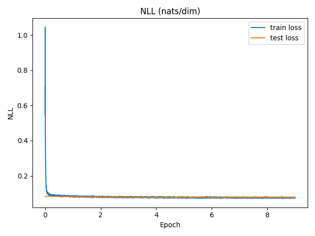
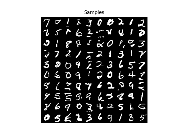
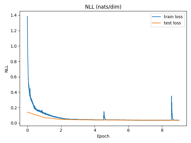
You will need to train the model using a GPU. You can import the source code into Google Colab and run the script in there. After the model finishes training, binary_nll.png and binary_samples.png can be found in the output/ directory. Below are those images after training the model for 10 epochs.

4.0 Pixel CNN Color Images

Now we will use the above modules to train a Pixel CNN on colored images. Unfortunately, my repo does not have enough storage to store the mnist_colored.pkl dataset but you can obtain this dataset from the Berkeley Deep Unsupervised Learning repo by unzipping deepul/homeworks/hw1/data/hw1_data.zip. A given image within in this dataset is of shape (28, 28, 3) and a given pixel takes on a value between [0, 3]. We will reuse a lot of the modules we already built, but will need to create a new masked convolution module which is reviewed in the next section.

4.1 Masked Convolution Color Images

Below is how the original paper defines Mask A and B for colored images.

In the case of type A, this means:

Similar to the toy example in section 3.1.1, assume we have an input image of 3x5x5, kernel size of 3x3 and 3 filters. In this setting the convolution weight matrix, W, would be of shape (3, 3, 3, 3) = (n_filters, in_channels, kernel_height, kernel_width). W[0, :, :, :], W[1, :, :, :] and W[2, :, :, :] are in charge of auto-encoding the R, G and B channels of the input image, respectively. As a result, the mask, M, under type A masked convolution would be as followed:

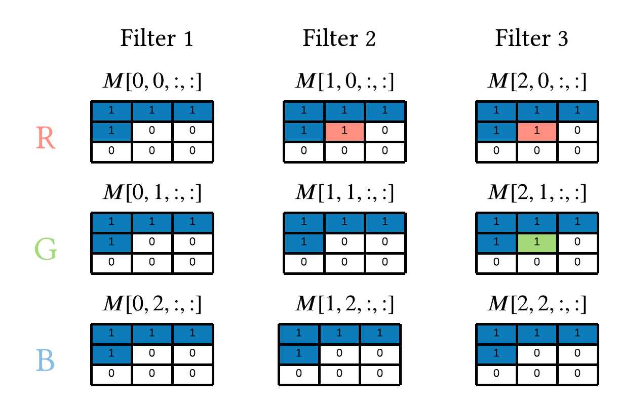
We notice Filter 1 zeros out everything but the context pixels because \(h^1_{i,R}\) is only a function of the context. Filter 2 zeros out everything but the context and \(x_{i,R}\). Finally, Filter 3 zeros out everything but the context, \(x_{i,R}\), and \(x_{i,G}\).

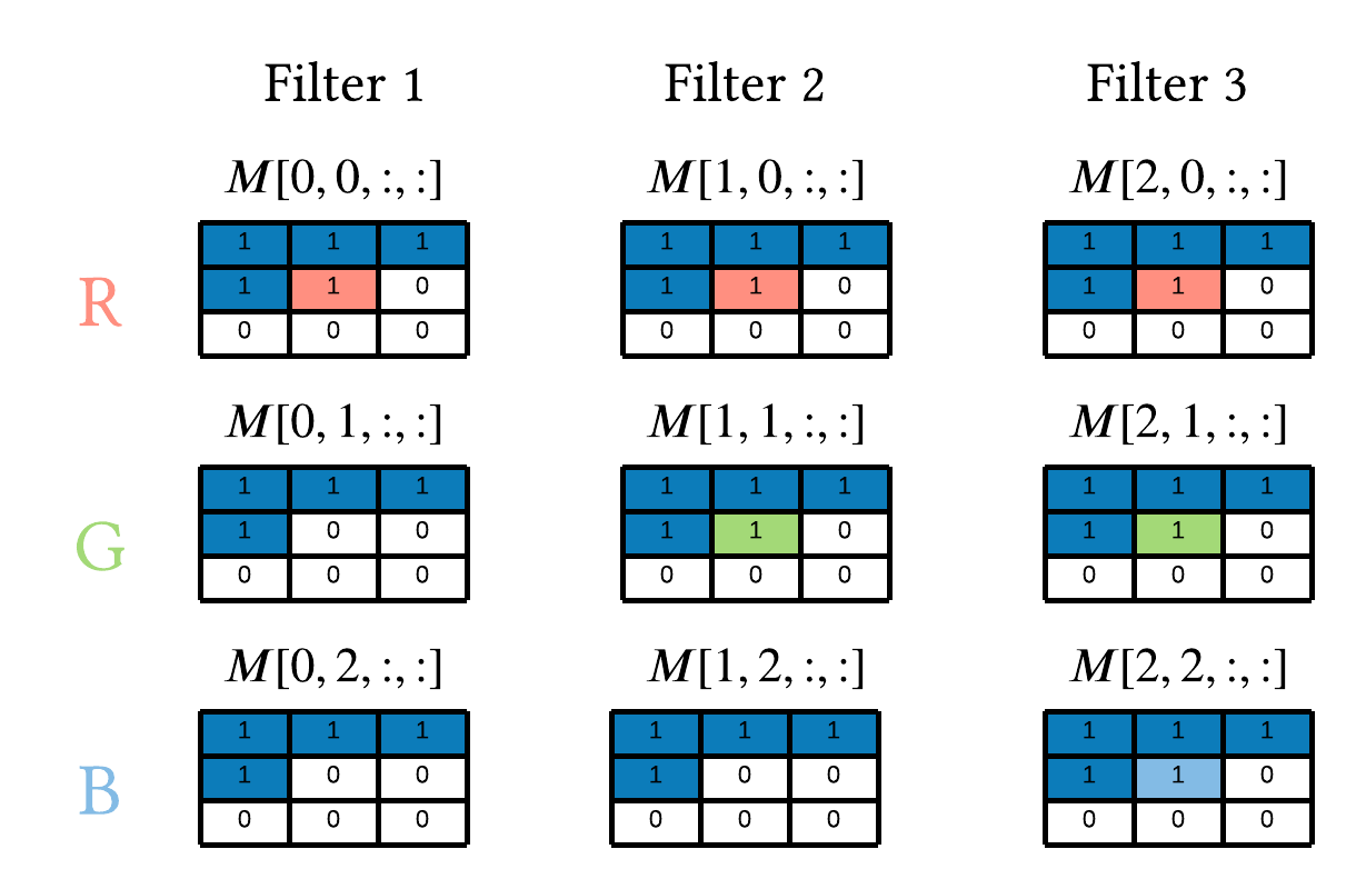
Next we have the mathematical representation of Mask B based off Figure 7:

Where the corresponding image is below.

4.2 Handling Large Input Channels and Filters

Now we need to generalize the above to cases where the number of model filters is greater than 3. Assume we train our model to have 120 filters at each convolution in the network. As a result, each hidden layer, \(\pmb{h}^l\), will have a tensor shape of (bsize, 120, 28, 28). What we do is split the input channels into 3 equal thirds, so \(\pmb{h}^l\)[:, 0:40, :, :] are Red channels, \(\pmb{h}^l\)[:, 40:80, :, :] are Green channels and \(\pmb{h}^l\)[:, 80:, :, :] are Blue channels. Furthermore, Filters 0-39, 40-79 and 80-120 are in charge of the Red, Green and Blue channels, respectively. In the of mask type B Filters 0-39, 40-79 and 80-120 would be similar to to Filters 1, 2 and 3 in Figure 8, respectively. Below is the Pytorch implementation.

class MaskedConv2dColor(MaskedConv2dBinary):
    def __init__(self, m_type, in_channels, out_channels, kernel_size, padding):
        super().__init__(m_type, in_channels, out_channels, kernel_size, padding)
        in_idx = in_channels // 3
        out_idx = out_channels // 3

        if m_type=='A':
            # allow R channels on 2nd third filters
            self.mask[out_idx:out_idx*2, :in_idx, kernel_size//2, kernel_size//2] = 1
            # allow R and G channels on 3rd third filters
            self.mask[out_idx*2:, 0:in_idx*2, kernel_size//2, kernel_size//2 ] = 1
        else:
            # zero out the middle pixel across all input channels and filters
            self.mask[:, :, kernel_size//2, kernel_size//2] = 0
            # allow R channels on the 1st third filters
            self.mask[:out_idx, :in_idx, kernel_size//2, kernel_size//2] = 1
            # allow R and G channels on the 2nd third filters
            self.mask[out_idx:out_idx*2, 0:in_idx*2, kernel_size//2, kernel_size//2] = 1
            # allow R, G and B channels on the 3rd third filters
            self.mask[out_idx*2:, :, kernel_size//2, kernel_size//2] = 1

conv_b = MaskedConv2dColor('B', 120, 120, 7, 3)
print(conv_b.mask.shape)
print(conv_b.mask[50, [10, 50, 90], :, :])

Output:

torch.Size([120, 120, 7, 7])
tensor([[[1., 1., 1., 1., 1., 1., 1.],
            [1., 1., 1., 1., 1., 1., 1.],
            [1., 1., 1., 1., 1., 1., 1.],
            [1., 1., 1., 1., 0., 0., 0.],
            [0., 0., 0., 0., 0., 0., 0.],
            [0., 0., 0., 0., 0., 0., 0.],
            [0., 0., 0., 0., 0., 0., 0.]],

        [[1., 1., 1., 1., 1., 1., 1.],
            [1., 1., 1., 1., 1., 1., 1.],
            [1., 1., 1., 1., 1., 1., 1.],
            [1., 1., 1., 1., 0., 0., 0.],
            [0., 0., 0., 0., 0., 0., 0.],
            [0., 0., 0., 0., 0., 0., 0.],
            [0., 0., 0., 0., 0., 0., 0.]],

        [[1., 1., 1., 1., 1., 1., 1.],
            [1., 1., 1., 1., 1., 1., 1.],
            [1., 1., 1., 1., 1., 1., 1.],
            [1., 1., 1., 0., 0., 0., 0.],
            [0., 0., 0., 0., 0., 0., 0.],
            [0., 0., 0., 0., 0., 0., 0.],
            [0., 0., 0., 0., 0., 0., 0.]]])

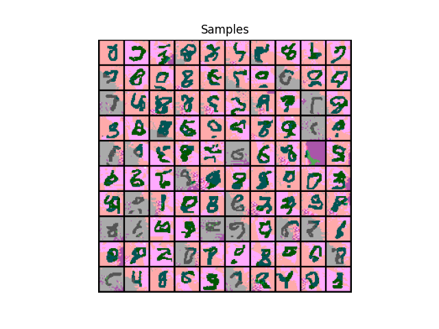
4.3 Color PixelCNN Results

Below will train our PixelCNN on colored mnist images.

Run:

python train.py --pickle data/mnist_colored.pkl --filters 120 --layers 8 --dev cuda --dist_size 4 --conv_class MaskedConv2dColor --lr 0.001 --nll_img_path output/color_nll.png --samples_img_path output/color_samples.png --save_path output/model_color.pt

Below are the results after training the model for 10 epochs.

5.0 Conclusion

Well, that is the PixelCNN. Hopefully this post provided you with some intuition on the model architecture that you couldn't find else where on the web. I highly encourage everyone to go and complete Berkeley's Deep Unsupervised Learning course. Assuming you are comfortable with independent learning, there is a lot of good content and they do highlight the present day state-of-the-art. If you liked this post, drop a line in the comments.

References

[1] Aaron Van Oord, Nal Kalchbrenner, and Koray Kavukcuoglu. Pixel recurrent neural networks. 48:1747–1756, 20–22 Jun 2016.
[2] University of California, Berkeley CS294-158-SP20 Deep Unsupervised Learning Spring 2020 https://sites.google.com/view/berkeley-cs294-158-sp20/home
[3] CS 294-158 Deep Unsupervised Learning GitHub Repository https://github.com/rll/deepul